I agree with Moop. The whole front (rear) mass is not located on one point at the center of the front (rear) axle. k2/ab is one of the "magic number " to master in transient.
 |

|
|
|
|

I agree with Moop. The whole front (rear) mass is not located on one point at the center of the front (rear) axle. k2/ab is one of the "magic number " to master in transient.
Claude Rouelle
OptimumG president
Vehicle Dynamics & Race Car Engineering
Training / Consulting / Simulation Software
FS & FSAE design judge USA / Canada / UK / Germany / Spain / Italy / China / Brazil / Australia
[url]www.optimumg.com[/u
I've had a look at Danny's suggestion at looking at the data in the CN-AY plane and extracting a trend from that. What I noticed immediately is that you get a completely different looking response for a hairpin, esses and a long sweeping bend. Some had positive trends, some negative and I thought that this isn't telling me what I want.
So, I've done a bit of research on this. In the absence of any track data thats shareable, I made a 2dof bicycle model in excel and ran it through some tests. The advantage of this approach is that I can calculate the stability index exactly using the model's mass, tyre and geometric data. The disadvantage is obviously that its not real data and for now it doesn't include tyre lag effects. Still, what I have seen is interesting.
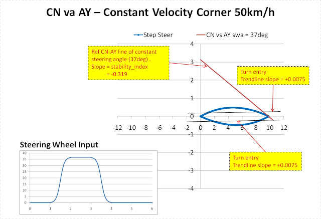
Using the bicycle model, I've done 3 operations which use a single nominal steering angle (37deg giving 1g) and speed (50kmh):
1. In the time domain I've done a few maneuvers (step steer, track corner, sinusoid 2Hz, frequency sweep all at 37deg swa) and had a look at the response in the N-Ay plane to see if I can extract a trend to call the stability index. I'm only looking at transients here.
2. I have created a reduced MMM diagram from the model showing a single line of const steering angle (37deg). The slope of this line is the stability index and it is -0.3188 for my model
3. I have calculated the stability index using a single formula. Again, I get -0.3188 for this model.
Basically what I found, which was my feeling from the start, is that different steering inputs from the driver give different responses on the N-Ay plane. So with a single model, with a single defined SI, I have seen that fitting a line to the CN-AY plane reponse doesn't give you what you want. The following examples will show this:
The step steer gives the best approximation of the stability index according to the calculation and in terms of the response in the CN-AY plane. I'd say this is because its the closest condition to a constrained MMM test. That is constant steering angle, so the yaw response comes primarily from the yawrate and sideslip effects. When I fit a line to the linear part of the CN-AY response, I get a number of -0.2939 which is reasonably close to the calculated SI of -0.3188
Next I gave it a steering input like you might see through a corner. So there is a transient section on corner entry, a steady section in the middle and a transient section on corner exit. In the response below I fitted a curve to both of the transient sections independantly and for both I curiously got identical numbers of +0.0075. Obviously not very well related to the stability index, but interestingly, the CN-AY reponse remains bounded by the single MMM line.
Next test, a sinusoidal input at constant velocity. Someting like you might see in silverstone through Maggots, Becketts but at a higher frequency (2Hz). Here its possible to appreciate some trend (trendline slope of -0.0193). Again its not equal to the stability index, BUT it does run tangent to it. So like the previous test, it is bounded by the single MMM line.
Finally I did a frequency sweep. This gave the coolest looking plot which had no trend at all but again seems perfectly bounded by the MMM line.
So, my conclusion so far is that the transient response you see on the CN-AY plane IS related to the stability index, BUT its not as simple as fitting a line to the data. I think I've shown here that with one car, one steering angle and one speed, you get totally different CN-AY reponses depending on what kind of steering input you give.
I think once you add in other realities such as braking/acceleration effects on speed and load transfer as well as tyre lag and non linear effects it would be pretty dangerous to fit a curve to the CN-AY plot and call it the stability index.
Tim
P.S. Sorry for not labelling my plot axes.
P.P.S Actually I'm not really sorry...
Tim
Last edited by Tim.Wright; 10-13-2013 at 03:22 PM.
Take the results from the chirp steer input to your model and process the Ay by steer and the Yaw Velocity by steer data to produce the transfer function summary in Bode form (Gain and Phase vs frequency). Then compute the phase margins for each and you will have a reliable stability metric because THAT'S WHAT A PHASE MARGIN IS).
Now change the model parameters and produce families of vehicles which have the same gain (ay by steer), the same understeer, the same rear cornering compliance and even 3 different values of rear roll-steer (steer by roll: deg/deg) [as in +.05, 0.0 and -.05]. The different roll steers will require you to recomputed the effective tire cornering stiffnesses in order to maintain the same rear cornering compliance for that family of runs.
When you compute the phase information for these combinations , the results will all be in Control System Engineering sense.
The only trick is to lump the front and rear tire and suspension parameters into cornering compliance units (I could post some of these for you if you can't figure it out).
Its so much easier and elegant when you use engineering tactics instead of IT or here-say methods.
To tackle the nonlinear effects, there are several alternative procedures:
1) Localized linearity: run the same play as for the linear model, except use the chirp steer signal running between 34 to 39 degrees of steer.
2) Us the Bendat and Piersol technique of running the results thru an inverse filter having the reverse characteristics of your nonlinearity (most probably them there tars). Since they are softening springs, the inverse tire model method is a classroom course first homework assignment. They wrote an entire book on this and I was fortunate to attend a class taught by these two guys on how to it works. I've enclosed the book details for those of you who can only text or tweet thus far in your educational resume'.
3) Run the fully nonlinear model results data through the FR test post processing and find out how disappointing the difference is between linear vehicles and non-linear vehicles in the frequency domain (except for one special detail). Again, all the nonlinearities in vehicle handling are (or better well should be) stiffening or softening springs. Anything else produces angry tires, angry drivers and angry owners (but happy fans and spectators).
If you say you are an Engineer, but use religion to explain your results, make sure you blow your whistle at every intersection crossing.
Thanks Bill, I will look into this when I get a few more spare minutes.
I have done something like the local linearised method already with a thesis student at my old uni. It was not in a dynamic model but it had nonlinear tyres. From what I had seen so far (its still in progress) there can be a reasonable difference between the behaviour in the linear range and at the limit.
Also, I had started the discussion because Im interested to see if there is a way to quantify stability using only track data. Here you generally don't have a tyre model to use as reference and no slip angle measurement. And your input is not a perfect chirp signal so you cant post process it using fft methods.
So for me there is still a gap for a lot more discussion.
Hey Guys,
Many thanks for contributing to this excellent discussion. There are few things I'd like to throw in and clarify,
First things first Tim - excellent work. It's really good to see some good analysis here. Let me throw in some observations and clarifications. Firstly the calculation of Stability Index via tyre data is an excellent start. It doesn't give you the exact answer but it tells you what to expect and this in of itself is a good thing.
Just with regards to what you said about Yaw moment vs lateral acceleration the overall curve fit is a tool to get you going but in reality you do have to dig a bit deeper which is precisely what you have done. As I stated in my last post about the Stability Index it is a measure of car stability that will change with the car conditions. The variation you got in the chicane result didn't surprise me at all. The thing that makes Race car vehicle dynamics so tricky is that your inputs have a fundamental impact on the characteristics of the car. Hence why they are going to vary. Let me give you a good case in point. When I was analysing some F3 data a while ago when I plotted Yaw moment vs lateral acceleration. When the g was low the slope was nice and linear indicating the car had good stability. As we approached peak cornering conditions the plot started to go all over the place since this was a particular bumpy circuit. This was a strong indication we had hit unstable behaviour. The give away was comparing actual to Neutral steer because as we got closer to the limit the neutral and steer lines where crossing in and out indicating unstable behaviour. Consequently I always use these two tools in concert with each other and I use the initial curve fit to get me going. I trust this makes sense.
Also just for my reference could you just clarify what your axes are. I found that bit just a bit confusing. Also too feel free to email me your results so we may have a more detailed discussion. I won't be able to respond this week because I'm tied up at time attack at Eastern Creek.
Moop - I would strongly suggest you double check your numbers. That little equation I put forward to approximate Yaw moment I've seen in use on many formula from V8 Supercars, GP2 and F3. I have lost count of the number of race engineers I know who have used this in anger as a sanity check to tell them what the car is doing . Granted this would break down in extreme cases of structural flexibility but if your at this point your throwing out the car anyway so it's a moot point.
Claude - My friend this is no magic number. The stability index is a measure of car stability at a particular point in time. It's up to the end user to determine what to do with it.
Keep up the good work guys. For those of you in the U.S I'm tending towards giving a mini seminar at this at PRI.
All the Best
Danny Nowlan
Director
ChassisSim Technologies
Hey Guys,
On another note, I just thought I'd give you another taster about what I'll be talking about at the simulation bootcamp in Europe and PRI in December at Lap Time Simulation 101,
http://www.chassissim.com/blog/chass...ith-chassissim
I'm looking forward to seeing you all there.
All the Best
Danny Nowlan
Director
ChassisSim Technologies
Tim. A Datron optical sideslip sensor is the most widely used xducer in the U.S. field. I have seen the telltale Datron lamp beam on the pavement during races when such measurements are forbidden. Oops.
Given a sideslip reading at centerline of the rear axle (best place to put it), this along with corrected lateral acceleration directly measures the vehicle's rear cornering compliance. You can also create a Math channel for the c.g. sideslip angle and a situation for which this signal is zero is a special case in vehicle dynamics. Called the Tangent Speed (because the vehicle is tangent to the turning circle path), the higher the Tangent Speed, the lower the rear cornering compliance. And, knowing this speed allows you to compute the rear cornering compliance just from vehicle geometric parameters. From this you can ascertain the tire stiffness at that trim by knowing a bit about the rear chassis compliances. In a racing vehicle, there ought not to be very much deflection steer or rear roll steer so the tire properties can be easily obtained or verified. Nothing like a K&C test to fill in these missing suspension parameters.
The goal of your test session would be to measure the tangent speed for every change in trial settings. The highest number speed is the best value. Of course the can be ugly, but if the number is high and the controllability is low (measure its Yaw rate by Steer Coherence). then you also know that the 'problems is at the front end. Best results come from a steering torque sensor because a 'feeling' driver will be in a moment control dialog with the car. Poor yaw velocity by steer torque coherence with also point out that friction is not your friend any more.
I believe I pointed out earlier that the FFT of Lateral Acceleration - Yaw Velocity phase information ( I call it the "RAY function") graphed vs. frequency will lie on a curve whose initial slope can also produce the vehicle's rear cornering compliance (rear axle axle sideslip angle) metric. Since there may be scale and other instruments snafus in your D.A. box, its pretty hard to screw up the time base, so this phase metric will be pretty freakin' accurate.
Now all you need is a constant radius portion of the track or test area and and a driver able to run a reasonable speed sweep through it. BTW: this is an I.S.O. test procedure. The Math functions for it are printed in the I.S.O. document as I recall.
You need to pat attention to more than yaw velocity because a high speed vehicle should be sidesliping a lot more than turning. And, turning more at low speeds. Even the Zamboni driver at my hockey rink knows this....
Tim,Originally posted by Tim:
I made a 2dof bicycle model in excel and ran it through some tests. The advantage of this approach is that I can calculate the stability index exactly using the model's mass, tyre and geometric data. The disadvantage is obviously that its not real data and for now it doesn't include tyre lag effects. Still, what I have seen is interesting.
Using the bicycle model, I've done 3 operations which use a single nominal steering angle (37deg giving 1g) and speed (50kmh):
1. In the time domain I've done a few maneuvers (step steer, track corner, sinusoid 2Hz, frequency sweep all at 37deg swa) and had a look at the response in the N-Ay plane to see if I can extract a trend to call the stability index. I'm only looking at transients here.
2. I have created a reduced MMM diagram from the model showing a single line of const steering angle (37deg). The slope of this line is the stability index and it is -0.3188 for my model
3. I have calculated the stability index using a single formula. Again, I get -0.3188 for this model.
I have had a quick look through the MMM section in RCVD to remind myself about this stuff. (Doug, if anything wrong below, then please correct.)
1. It seems that this MMM approach is quite simplified (nothing wrong with that!) in that it is a bicycle model in pseudo-steady-state cornering (err..., at very large radius). This means that any Yaw Moment (= Yaw Couple!!!) "N" acting on the car DOES NOT cause a Yaw acceleration. So no Yaw MoI is included in this model, since it does not matter for this type of analysis. So not really good for "looking at transients"...
2. Minor point, but Milliken's "CN" is a non-dimensionalised "coefficient" of the Yaw force (= N/Wl), and their AY is also non-dimensionalised (= Ay/g, so in units of "G" = ~0-2 for typical FSAE cars). However, even in this one chapter there seemed to be some variability on the labelling of axes.
3. Milliken's "stability index" seems to be dCN/dAY for FIXED front steer angle, but varying car side-slip angle (= beta), measured at CN = 0.
4. The whole MMM map, similar to your last picture of a frequency sweep, gives the maximum "performance envelope" of the car (given the limits of this simple model). The baseline "stability index" at steer-angle = 0, side-slip-angle = 0, CN = 0, and AY = 0, is a diagonal line with similar slope to the one you show, but passing through the origin. The "limit performance" of the car is indicated by the right-hand corner of the diamond shaped map. If this corner is below the AY-axis, then understeer at the limit. If above AY-axis, then oversteer at the limit.
~~~o0o~~~
Anyway, I am curious to know more details about your analysis.
1. Do you include Yaw MoI, or are you as per the MMM?
2. What are the labels of your axes?
3. What formula did you use to calculate the stability index exactly (I suspect this should give the same as 3 above)?
Finally, I remind anyone doing this MMM sort of analysis that its pseudo-static nature, with no account of Yaw MoI, gives it VERY LIMITED APPLICABILITY in FSAE conditions (which are mostly "transients").
Z
Z -- The MMM analysis can be arbitrarily detailed: Some of the early examples in Chapter 8 use a bicycle model, possibly using tire data based on pair analysis (Chapter 7). The later examples in C.8 include detailed tire data, aero data and measured K&C. MMM is a simulation of a constrained test (like wind tunnel tests and aircraft "statics") so there is no yaw acceleration, but, the N (or CN) would most certainly produce a yaw acceleration if the constraint were removed.Originally Posted by Z

You might want to look at Table 8.4 which lists some of the different diagrams (plotted on different axes) and how they relate to different kinds of maneuvers.
Like any tool, it has strengths and weaknesses. One strength is the ability (after some practice by the user) to see the whole performance envelope of the car, which makes it easy to look at many of the big questions in preliminary design. A major weakness (in terms of commercial acceptance!) is that it typically takes a month or two of use and training to get familiar with the concepts and learn to interpret the results...
Erik,
I will give a more detailed answer later when I'm back home but I agree with your points above. The MMM line was generated using the basic sum of forces and sum of moments equations (using the control derivatives) and with a sweep of slip angle (I think I did a range of =-3deg). BUT the one manipulation is that in these equations I have replaced yawrate with Ay/v. So yes, this does make is pseudo steady state like you mentioned. In fact, you can see in the step steer results, the vehicle response asymptotes towards the MMM line as it reaches steady state (i.e. when the condition r = Ay/v actually becomes true).
Im not sure its valid to talk about limits here because I'm using a linear tyre model.
The axes are:
Vert: CN = (yaw_moment/(wheelbase x mass))
Hor: AY = lateral_acceleration/9.81
 Posting Permissions
 Reply With Quote